Compression Artifact localization as a Semantic Segmentation task
Let’s start with compression artifact definition — a noticeable distortion of media caused by the application of lossy compression.
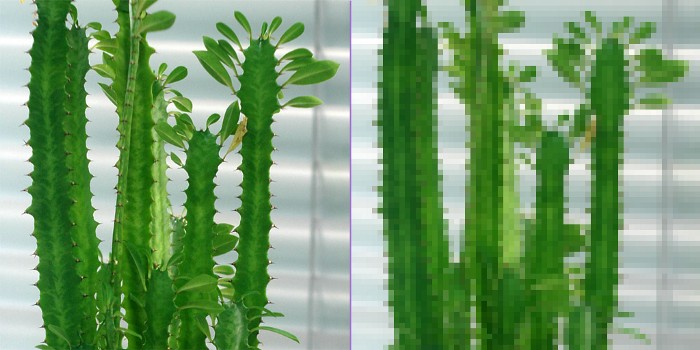
The scope of deep learning algorithms is growing every year. For example, in medicine, deep learning helps to segment images into cancerous and non-cancerous sections. Similarly, our task is to segment images into sections with and without compression artifact.
The application area of our task is quite wide. It can be integrated into live streaming monitoring systems and also can be used in video quality assurance.
Our task is also closely related to another popular computer vision task — “Single Image super resolution”. The problem is that directly performing image super-resolution (SR) to an image with a huge compression artifact segment would also simultaneously magnify the blocking artifacts, resulting in unpleasant visual experience. That’s why the information about compression artifact’s appearance in an image will be very useful and helpful.
Method
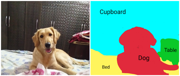
As I mentioned above, we need to segment images into sections with and without compression artifact. This is where Semantic Segmentation shines. Semantic Segmentation refers to the process of linking each pixel in an image to a class label.
In our task these labels include four compression-based distortion types:
- H.264 compression
- MJPEG compression
- Wavelet compression
- HEVC compression
Thereby for each pixel it will be predicted whether it belongs to one of these 4 classes or whether it is a pixel without an artifact.
If you are familiar with deep learning, you might also have heard about Instance Segmentation and wondering why we don’t use it.
So, let’s take a look at the differences between Semantic and Instance Segmentation.
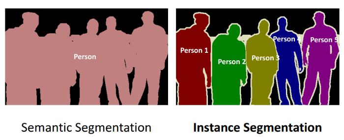
Different instances of the same class are segmented individually in Instance Segmentation. We can see in the above image that different instances of the same class have been given different labels. Since this kind of information is redundant for us, we don’t use the Instance Segmentation.
Dataset
To solve this task, CSIQ dataset was chosen. This dataset consist of 12 high-quality reference videos and 216 distorted videos from six different types of distortion. For each reference video, I applied one of six types of distortion at three different levels of distortion. The distortion types comprise of four compression-based distortions and two transmission-based distortions. I picked only compression-based distortions:
- H.264 compression (H.264)
- HEVC/H.265 compression (HEVC)
- Motion JPEG compression
- Wavelet-based compression using Snow codec (SNOW)
I have fully distorted images in CSIQ dataset but for the task at hand I need to train the model to segment an image into an area with and without artifact. That’s why I need partly distorted images in our dataset.
The training dataset was created by the following steps:
- Taking a reference image
- Taking a corresponding distorted image
- Generating a random rectangle area and replacing such areas in the original image with a distorted one.
After following these steps we have partly distorted images and masks.

Results
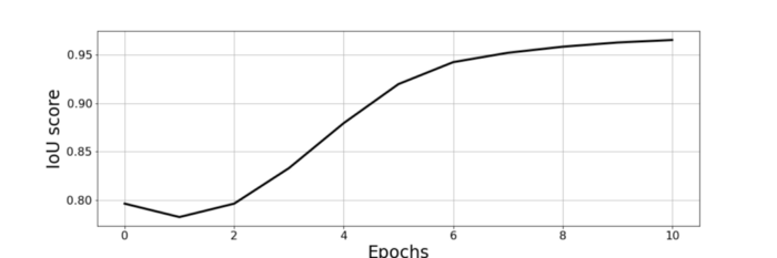
Training progress
After the first epoch, IOU score was equal to 0.79 which is already a quite decent result. The dataset size was 12.000 samples, it took about 11 hours to learn 10 epochs with batch size equal to 8. The final IOU score reached 0.97.
Test
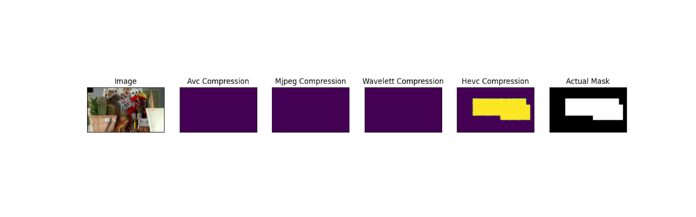
Test on validation data from CSIQ:
After we’ve trained our model we need to test it with validation data from CSIQ dataset.
The first sample is the image partly distorted with HEVC compression artifacts.

The second sample is the image partly distorted with MJPEG compression artifacts.

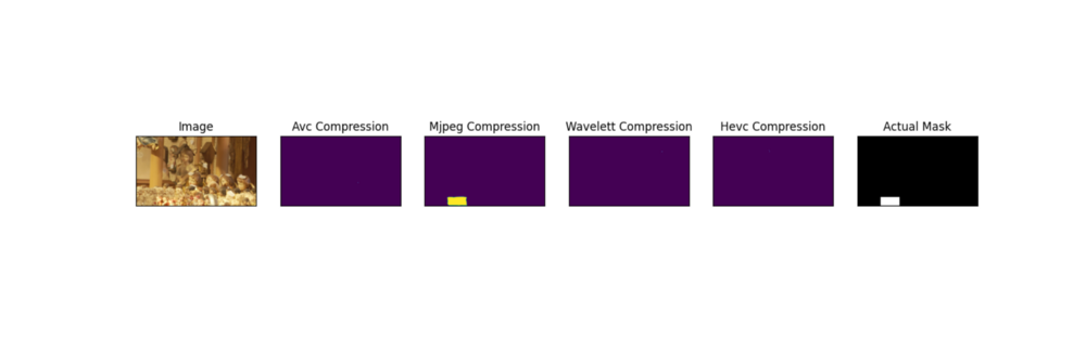
As we can see, the model correctly classifies the codec type and segments the distorted area, very close to the actual mask.
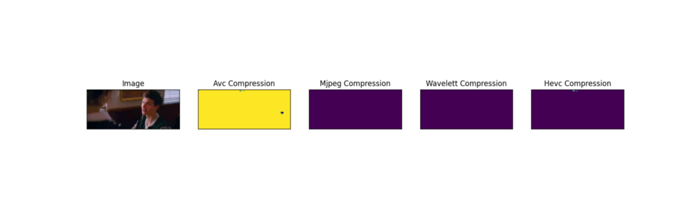
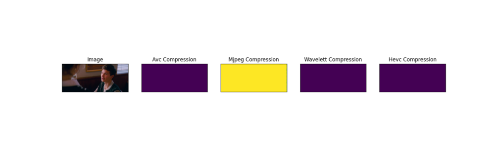
The model is also tested on “Baby Driver” trailer compressed with different video codecs . For this test, the trailer was compressed with a purposely low bitrate (0.1 megabits — empirically selected value) in order to introduce compression artifacts. In contrast to the test on validation data from the CSIQ dataset, here the entire frame has compression artifacts.


Conclusion
As a result of this work, we have obtained a tool that can detect not only the presence of compression artifacts in an image, but also localize them and determine video codec type which was used for compression.
Interested in machine learning? Explore our website.